Tidy Tuesday Exercise

Load Necessary packages from library

Getting the data #Install tidytuesdayR which will load all datasets needed #install/download other needed packates

library(tidytuesdayR)

Warning: package 'tidytuesdayR' was built under R version 4.2.2

library(plyr)
library(dplyr)

Warning: package 'dplyr' was built under R version 4.2.2

Attaching package: 'dplyr'

The following objects are masked from 'package:plyr':

    arrange, count, desc, failwith, id, mutate, rename, summarise,
    summarize

The following objects are masked from 'package:stats':

    filter, lag

The following objects are masked from 'package:base':

    intersect, setdiff, setequal, union

library(ggplot2)

Warning: package 'ggplot2' was built under R version 4.2.2

library(here)

here() starts at C:/Data/GitHub/MADA23/betelihemgetachew-MADA-portfolio2

Attaching package: 'here'

The following object is masked from 'package:plyr':

    here

library(tidyverse)

Warning: package 'tidyverse' was built under R version 4.2.2

── Attaching packages
───────────────────────────────────────
tidyverse 1.3.2 ──

✔ tibble  3.1.8     ✔ purrr   0.3.4
✔ tidyr   1.2.0     ✔ stringr 1.5.0
✔ readr   2.1.2     ✔ forcats 0.5.1

Warning: package 'stringr' was built under R version 4.2.2

── Conflicts ────────────────────────────────────────── tidyverse_conflicts() ──
✖ dplyr::arrange()   masks plyr::arrange()
✖ purrr::compact()   masks plyr::compact()
✖ dplyr::count()     masks plyr::count()
✖ dplyr::desc()      masks plyr::desc()
✖ dplyr::failwith()  masks plyr::failwith()
✖ dplyr::filter()    masks stats::filter()
✖ dplyr::id()        masks plyr::id()
✖ dplyr::lag()       masks stats::lag()
✖ dplyr::mutate()    masks plyr::mutate()
✖ dplyr::rename()    masks plyr::rename()
✖ dplyr::summarise() masks plyr::summarise()
✖ dplyr::summarize() masks plyr::summarize()

library(janitor)

Warning: package 'janitor' was built under R version 4.2.2

Attaching package: 'janitor'

The following objects are masked from 'package:stats':

    chisq.test, fisher.test

library(reshape)

Warning: package 'reshape' was built under R version 4.2.2

Attaching package: 'reshape'

The following objects are masked from 'package:tidyr':

    expand, smiths

The following object is masked from 'package:dplyr':

    rename

The following objects are masked from 'package:plyr':

    rename, round_any

Import Data

#load the tidytuesday data

tuesdata<-tidytuesdayR::tt_load('2023-02-14')

--- Compiling #TidyTuesday Information for 2023-02-14 ----

--- There is 1 file available ---

--- Starting Download ---

    Downloading file 1 of 1: `age_gaps.csv`

--- Download complete ---

#Read the specific age gaps dataset

age_gaps<-tuesdata$age_gaps

Getting Familiar with the data

#Ensure your data loaded correctly and understanding the data structure

colnames(age_gaps)

 [1] "movie_name"         "release_year"       "director"          
 [4] "age_difference"     "couple_number"      "actor_1_name"      
 [7] "actor_2_name"       "character_1_gender" "character_2_gender"
[10] "actor_1_birthdate"  "actor_2_birthdate"  "actor_1_age"       
[13] "actor_2_age"       

view(age_gaps)

glimpse(age_gaps)

Rows: 1,155
Columns: 13
$ movie_name         <chr> "Harold and Maude", "Venus", "The Quiet American", …
$ release_year       <dbl> 1971, 2006, 2002, 1998, 2010, 1992, 2009, 1999, 199…
$ director           <chr> "Hal Ashby", "Roger Michell", "Phillip Noyce", "Joe…
$ age_difference     <dbl> 52, 50, 49, 45, 43, 42, 40, 39, 38, 38, 36, 36, 35,…
$ couple_number      <dbl> 1, 1, 1, 1, 1, 1, 1, 1, 1, 1, 1, 1, 1, 1, 1, 1, 1, …
$ actor_1_name       <chr> "Ruth Gordon", "Peter O'Toole", "Michael Caine", "D…
$ actor_2_name       <chr> "Bud Cort", "Jodie Whittaker", "Do Thi Hai Yen", "T…
$ character_1_gender <chr> "woman", "man", "man", "man", "man", "man", "man", …
$ character_2_gender <chr> "man", "woman", "woman", "woman", "man", "woman", "…
$ actor_1_birthdate  <date> 1896-10-30, 1932-08-02, 1933-03-14, 1930-09-17, 19…
$ actor_2_birthdate  <date> 1948-03-29, 1982-06-03, 1982-10-01, 1975-11-08, 19…
$ actor_1_age        <dbl> 75, 74, 69, 68, 81, 59, 62, 69, 57, 77, 59, 56, 65,…
$ actor_2_age        <dbl> 23, 24, 20, 23, 38, 17, 22, 30, 19, 39, 23, 20, 30,…

class(age_gaps)

[1] "spec_tbl_df" "tbl_df"      "tbl"         "data.frame" 

dim(age_gaps)

[1] 1155   13

summary(age_gaps)

  movie_name         release_year    director         age_difference 
 Length:1155        Min.   :1935   Length:1155        Min.   : 0.00  
 Class :character   1st Qu.:1997   Class :character   1st Qu.: 4.00  
 Mode  :character   Median :2004   Mode  :character   Median : 8.00  
                    Mean   :2001                      Mean   :10.42  
                    3rd Qu.:2012                      3rd Qu.:15.00  
                    Max.   :2022                      Max.   :52.00  
 couple_number   actor_1_name       actor_2_name       character_1_gender
 Min.   :1.000   Length:1155        Length:1155        Length:1155       
 1st Qu.:1.000   Class :character   Class :character   Class :character  
 Median :1.000   Mode  :character   Mode  :character   Mode  :character  
 Mean   :1.398                                                           
 3rd Qu.:2.000                                                           
 Max.   :7.000                                                           
 character_2_gender actor_1_birthdate    actor_2_birthdate     actor_1_age   
 Length:1155        Min.   :1889-04-16   Min.   :1906-10-06   Min.   :18.00  
 Class :character   1st Qu.:1953-05-16   1st Qu.:1965-03-25   1st Qu.:33.00  
 Mode  :character   Median :1964-10-03   Median :1974-07-30   Median :39.00  
                    Mean   :1960-09-07   Mean   :1971-01-29   Mean   :40.64  
                    3rd Qu.:1973-08-07   3rd Qu.:1982-04-07   3rd Qu.:47.00  
                    Max.   :1996-06-01   Max.   :1996-11-11   Max.   :81.00  
  actor_2_age   
 Min.   :17.00  
 1st Qu.:25.00  
 Median :29.00  
 Mean   :30.21  
 3rd Qu.:34.00  
 Max.   :68.00  

str(age_gaps)

spc_tbl_ [1,155 × 13] (S3: spec_tbl_df/tbl_df/tbl/data.frame)
 $ movie_name        : chr [1:1155] "Harold and Maude" "Venus" "The Quiet American" "The Big Lebowski" ...
 $ release_year      : num [1:1155] 1971 2006 2002 1998 2010 ...
 $ director          : chr [1:1155] "Hal Ashby" "Roger Michell" "Phillip Noyce" "Joel Coen" ...
 $ age_difference    : num [1:1155] 52 50 49 45 43 42 40 39 38 38 ...
 $ couple_number     : num [1:1155] 1 1 1 1 1 1 1 1 1 1 ...
 $ actor_1_name      : chr [1:1155] "Ruth Gordon" "Peter O'Toole" "Michael Caine" "David Huddleston" ...
 $ actor_2_name      : chr [1:1155] "Bud Cort" "Jodie Whittaker" "Do Thi Hai Yen" "Tara Reid" ...
 $ character_1_gender: chr [1:1155] "woman" "man" "man" "man" ...
 $ character_2_gender: chr [1:1155] "man" "woman" "woman" "woman" ...
 $ actor_1_birthdate : Date[1:1155], format: "1896-10-30" "1932-08-02" ...
 $ actor_2_birthdate : Date[1:1155], format: "1948-03-29" "1982-06-03" ...
 $ actor_1_age       : num [1:1155] 75 74 69 68 81 59 62 69 57 77 ...
 $ actor_2_age       : num [1:1155] 23 24 20 23 38 17 22 30 19 39 ...
 - attr(*, "spec")=
  .. cols(
  ..   movie_name = col_character(),
  ..   release_year = col_double(),
  ..   director = col_character(),
  ..   age_difference = col_double(),
  ..   couple_number = col_double(),
  ..   actor_1_name = col_character(),
  ..   actor_2_name = col_character(),
  ..   character_1_gender = col_character(),
  ..   character_2_gender = col_character(),
  ..   actor_1_birthdate = col_date(format = ""),
  ..   actor_2_birthdate = col_date(format = ""),
  ..   actor_1_age = col_double(),
  ..   actor_2_age = col_double()
  .. )
 - attr(*, "problems")=<externalptr> 

names(age_gaps)

 [1] "movie_name"         "release_year"       "director"          
 [4] "age_difference"     "couple_number"      "actor_1_name"      
 [7] "actor_2_name"       "character_1_gender" "character_2_gender"
[10] "actor_1_birthdate"  "actor_2_birthdate"  "actor_1_age"       
[13] "actor_2_age"       

print(age_gaps)

# A tibble: 1,155 × 13
   movie_name    relea…¹ direc…² age_d…³ coupl…⁴ actor…⁵ actor…⁶ chara…⁷ chara…⁸
   <chr>           <dbl> <chr>     <dbl>   <dbl> <chr>   <chr>   <chr>   <chr>  
 1 Harold and M…    1971 Hal As…      52       1 Ruth G… Bud Co… woman   man    
 2 Venus            2006 Roger …      50       1 Peter … Jodie … man     woman  
 3 The Quiet Am…    2002 Philli…      49       1 Michae… Do Thi… man     woman  
 4 The Big Lebo…    1998 Joel C…      45       1 David … Tara R… man     woman  
 5 Beginners        2010 Mike M…      43       1 Christ… Goran … man     man    
 6 Poison Ivy       1992 Katt S…      42       1 Tom Sk… Drew B… man     woman  
 7 Whatever Wor…    2009 Woody …      40       1 Larry … Evan R… man     woman  
 8 Entrapment       1999 Jon Am…      39       1 Sean C… Cather… man     woman  
 9 Husbands and…    1992 Woody …      38       1 Woody … Juliet… man     woman  
10 Magnolia         1999 Paul T…      38       1 Jason … Julian… man     woman  
# … with 1,145 more rows, 4 more variables: actor_1_birthdate <date>,
#   actor_2_birthdate <date>, actor_1_age <dbl>, actor_2_age <dbl>, and
#   abbreviated variable names ¹​release_year, ²​director, ³​age_difference,
#   ⁴​couple_number, ⁵​actor_1_name, ⁶​actor_2_name, ⁷​character_1_gender,
#   ⁸​character_2_gender
# ℹ Use `print(n = ...)` to see more rows, and `colnames()` to see all variable names

Data Cleaning Checks

head(age_gaps)

# A tibble: 6 × 13
  movie_name     relea…¹ direc…² age_d…³ coupl…⁴ actor…⁵ actor…⁶ chara…⁷ chara…⁸
  <chr>            <dbl> <chr>     <dbl>   <dbl> <chr>   <chr>   <chr>   <chr>  
1 Harold and Ma…    1971 Hal As…      52       1 Ruth G… Bud Co… woman   man    
2 Venus             2006 Roger …      50       1 Peter … Jodie … man     woman  
3 The Quiet Ame…    2002 Philli…      49       1 Michae… Do Thi… man     woman  
4 The Big Lebow…    1998 Joel C…      45       1 David … Tara R… man     woman  
5 Beginners         2010 Mike M…      43       1 Christ… Goran … man     man    
6 Poison Ivy        1992 Katt S…      42       1 Tom Sk… Drew B… man     woman  
# … with 4 more variables: actor_1_birthdate <date>, actor_2_birthdate <date>,
#   actor_1_age <dbl>, actor_2_age <dbl>, and abbreviated variable names
#   ¹​release_year, ²​director, ³​age_difference, ⁴​couple_number, ⁵​actor_1_name,
#   ⁶​actor_2_name, ⁷​character_1_gender, ⁸​character_2_gender
# ℹ Use `colnames()` to see all variable names

#check for missing values

age_gaps[age_gaps==""]

<unspecified> [0]

#check the class for each column

sapply(age_gaps, class)

        movie_name       release_year           director     age_difference 
       "character"          "numeric"        "character"          "numeric" 
     couple_number       actor_1_name       actor_2_name character_1_gender 
         "numeric"        "character"        "character"        "character" 
character_2_gender  actor_1_birthdate  actor_2_birthdate        actor_1_age 
       "character"             "Date"             "Date"          "numeric" 
       actor_2_age 
         "numeric" 

#convert column classes as approporiate , it was fine but i did it anyways

age_gaps<-type.convert(age_gaps, as.is=TRUE)

#check if class is correct and appropriate

sapply(age_gaps, class)

        movie_name       release_year           director     age_difference 
       "character"          "integer"        "character"          "integer" 
     couple_number       actor_1_name       actor_2_name character_1_gender 
         "integer"        "character"        "character"        "character" 
character_2_gender  actor_1_birthdate  actor_2_birthdate        actor_1_age 
       "character"        "character"        "character"          "integer" 
       actor_2_age 
         "integer" 

#now lets check any values that are outliers age_difference variable

age_gaps$age_difference[age_gaps$age_difference %in% boxplot.stats(age_gaps$age_difference)$out] 

 [1] 52 50 49 45 43 42 40 39 38 38 36 36 35 35 34 34 34 34 33 33 33 32 32 32 32
[26] 32 32

#Capitalize variable values and Change male to Male and female to Female

age_gaps <- age_gaps %>%
  mutate(character_1_gender = case_when(
    character_1_gender == "man" ~ "Man",
    character_1_gender == "woman" ~ "Woman")) %>%
  mutate(character_2_gender = case_when(
    character_2_gender == "man" ~ "Man",
    character_2_gender == "woman" ~ "Woman"))

Explore the Data!

#now explore the data more by looking at historgram and boxplots

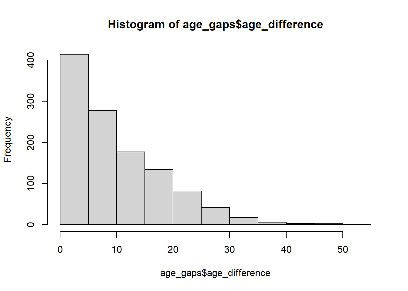
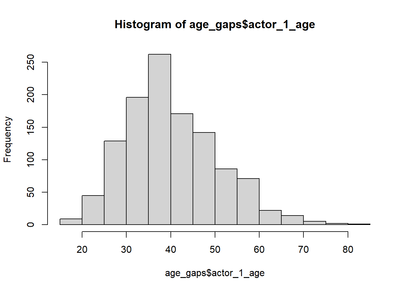
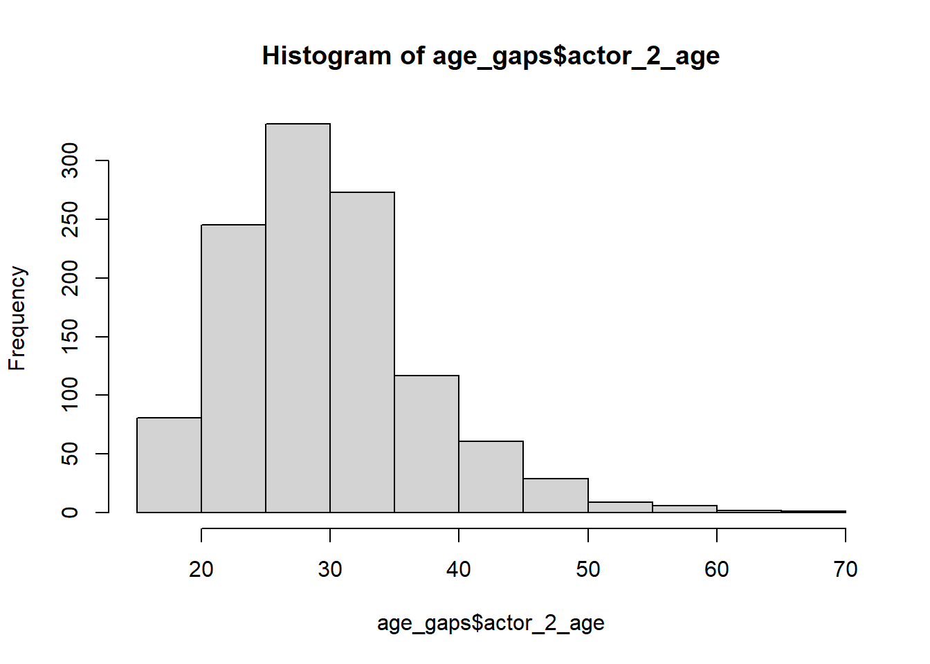
#The first histograms provides the distribution of the age difference in the sample and is right skewed. The second and third histograms provide the distribution of the age difference among the older actor and younger actor in the couples which seem to be normally distributed.

hist(age_gaps$age_difference)

hist(age_gaps$actor_1_age)

hist(age_gaps$actor_2_age)

#plot to check for patterns in terms of movie releases by Year

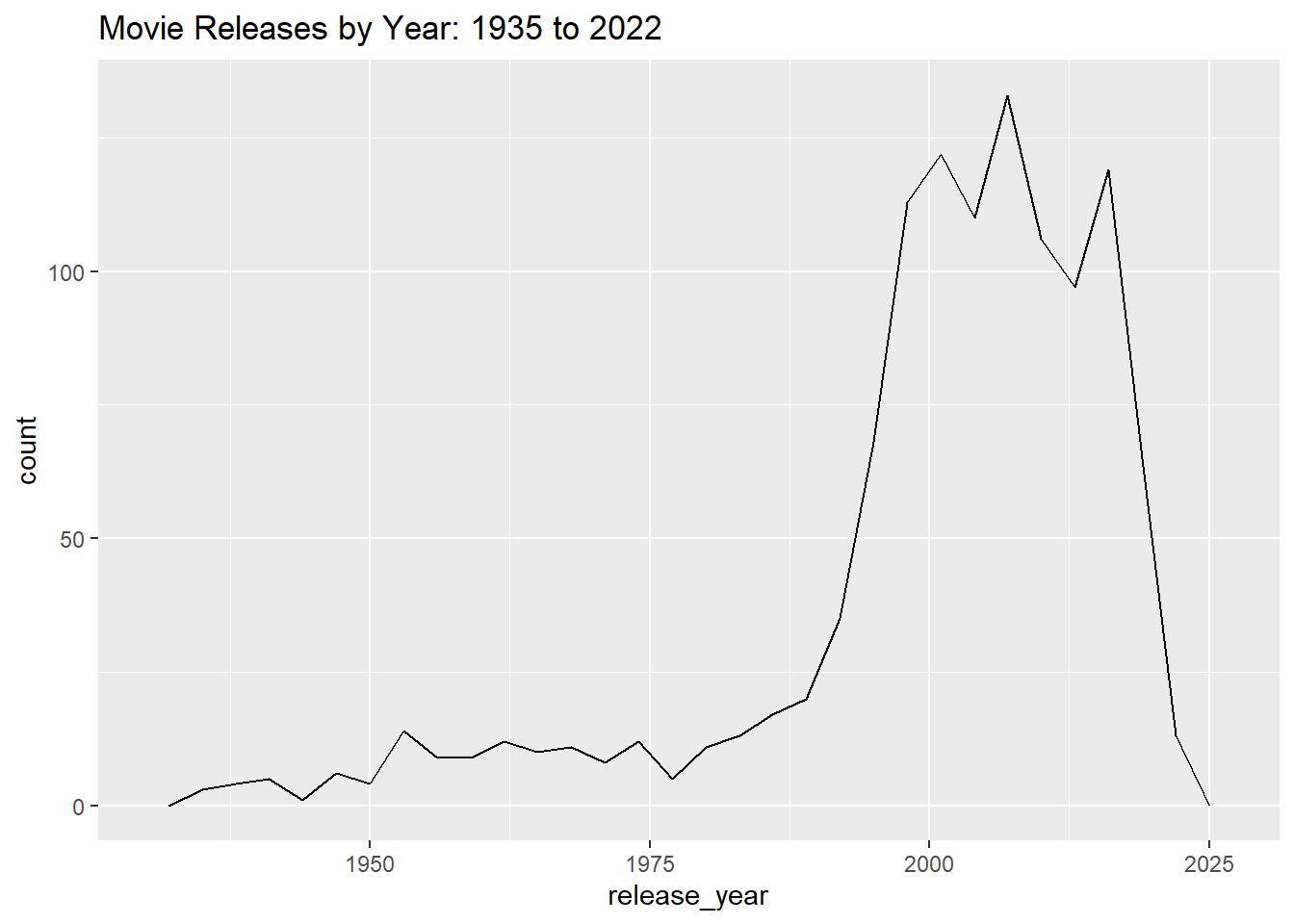
ggplot(age_gaps,aes(release_year))+ geom_freqpoly()+ggtitle("Movie Releases by Year: 1935 to 2022")

`stat_bin()` using `bins = 30`. Pick better value with `binwidth`.

#There was a surge in movie releases between the year 1985 to about 2000. After the 2000s while it still remained that high number of movies were releaed, there were a few highs and lows.

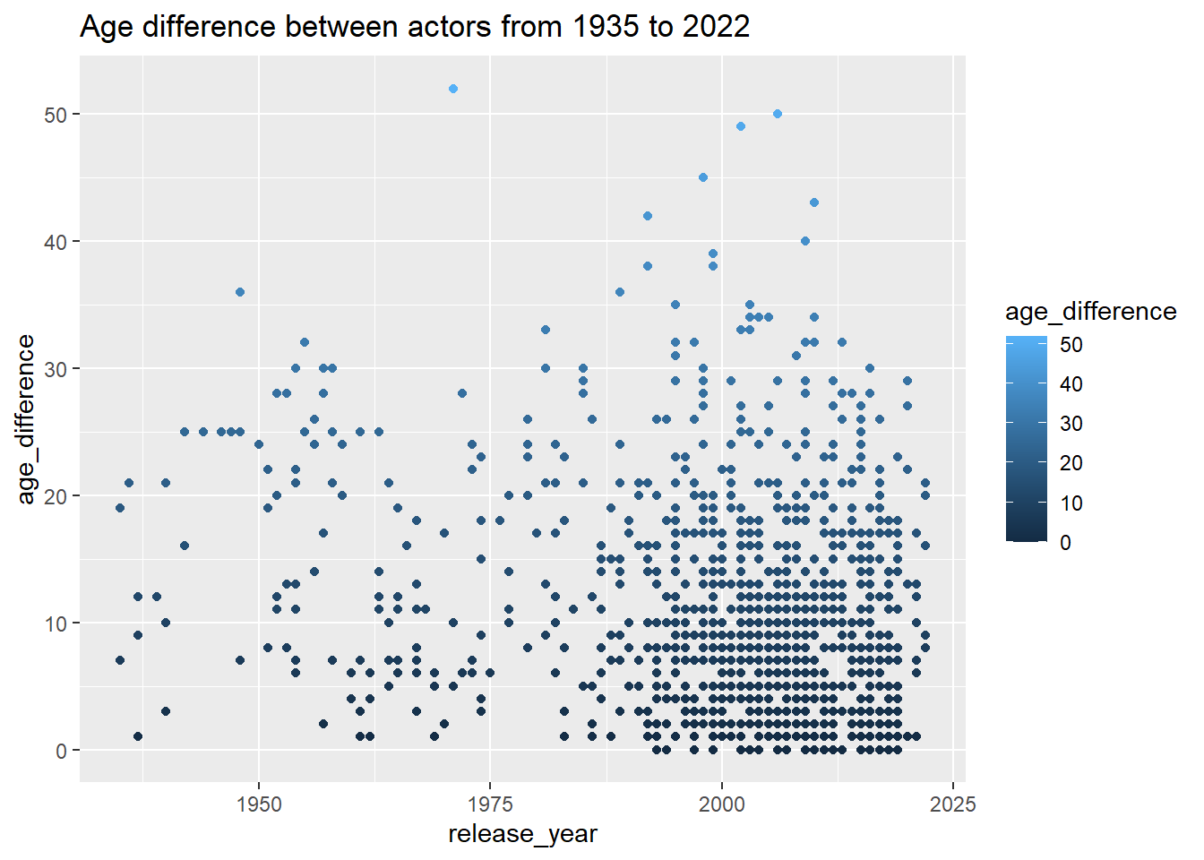
ggplot(data=age_gaps, aes(x=release_year, y=age_difference,col=age_difference))+geom_point()+ggtitle("Age difference between actors from 1935 to 2022")

#Mean and median age difference

meandata=mean(age_gaps$age_difference)
print(meandata)

[1] 10.42424

mediandata=median(age_gaps$age_difference)
print(mediandata)

[1] 8

Gender difference in the young and older group

Proportion of older actor by Gender

#Approx. 81% Men and 18% Woman were older

gender_table<-table(age_gaps$character_1_gender)
gender_table/sum(gender_table)

      Man     Woman 
0.8147186 0.1852814 

Proportion of younger actor by Gender

Approx. 18% Men and 81% Women were younger

gender_table<-table(age_gaps$character_2_gender)
prop.table(gender_table)

      Man     Woman 
0.1861472 0.8138528 

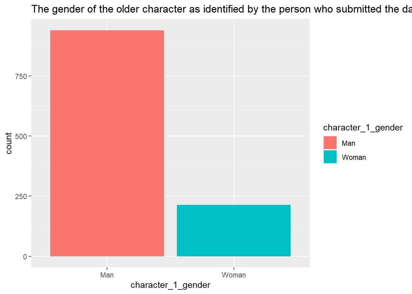
#Representing the above information in a bar chart ….

ggplot(age_gaps, aes(character_1_gender, ..count..))+geom_bar(aes(fill=character_1_gender), position="dodge")+ ggtitle("The gender of the older character as identified by the person who submitted the data for this couple")

Warning: The dot-dot notation (`..count..`) was deprecated in ggplot2 3.4.0.
ℹ Please use `after_stat(count)` instead.

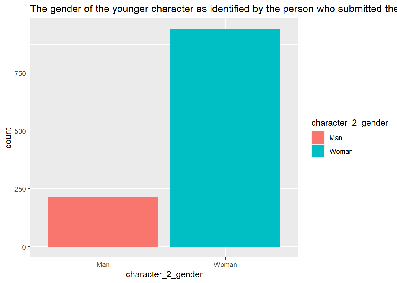
ggplot(age_gaps, aes(character_2_gender, ..count..))+geom_bar(aes(fill=character_2_gender), position="dodge")+ ggtitle("The gender of the younger character as identified by the person who submitted the data for this couple")

#Directors characteristics #director with the most releases.

age_gaps %>% group_by(director) %>% summarise(Freq=n()) %>% arrange(desc(Freq)) 

# A tibble: 510 × 2
   director          Freq
   <chr>            <int>
 1 Woody Allen         20
 2 John Glen           15
 3 Martin Scorsese     13
 4 Mike Newell         10
 5 Steven Spielberg    10
 6 David Fincher        9
 7 Dennis Dugan         9
 8 Guy Hamilton         9
 9 Mike Nichols         9
10 Nancy Meyers         9
# … with 500 more rows
# ℹ Use `print(n = ...)` to see more rows

Woody Allen, John Glen, Martin Scorsese, Mike Newell, Steven Spielberg have each released between 10-20 movies over the past 3 to 4 decades…

Notes

The data set was somewhat clean.There are 1155 observations with 13 variables. As far as the data, there are more men in the older actor group and more women in the young actor age group.The mean age difference is 10.4 years and the median age difference is 8 years. The age difference seemed to have decreased in recent years staying mostly between 0 to 20 years difference in the past 20 years. Last few decades there was a influx of movie releases.