Load necessary packages
Load necessary packages
library (broom.mixed)#for converting bayesian models to tidy tibbles
Warning: package 'broom.mixed' was built under R version 4.2.2
library (dotwhisker)#for visualizing regression results
Warning: package 'dotwhisker' was built under R version 4.2.2
Loading required package: ggplot2
Warning: package 'ggplot2' was built under R version 4.2.2
library (skimr) #for visualization
Warning: package 'skimr' was built under R version 4.2.2
library (here) #data loading/saving
here() starts at C:/Data/GitHub/MADA23/betelihemgetachew-MADA-portfolio2
library (dplyr)#data cleaning and processing
Warning: package 'dplyr' was built under R version 4.2.2
Attaching package: 'dplyr'
The following objects are masked from 'package:stats':

    filter, lag
The following objects are masked from 'package:base':

    intersect, setdiff, setequal, union
library (tidyr) #data cleaning and processing library (tidymodels) #for modeling
Warning: package 'tidymodels' was built under R version 4.2.2
── Attaching packages ────────────────────────────────────── tidymodels 1.0.0 ──
✔ broom        1.0.1     ✔ rsample      1.1.1
✔ dials        1.1.0     ✔ tibble       3.1.8
✔ infer        1.0.4     ✔ tune         1.0.1
✔ modeldata    1.1.0     ✔ workflows    1.1.3
✔ parsnip      1.0.4     ✔ workflowsets 1.0.0
✔ purrr        0.3.4     ✔ yardstick    1.1.0
✔ recipes      1.0.5
Warning: package 'dials' was built under R version 4.2.2
Warning: package 'infer' was built under R version 4.2.2
Warning: package 'modeldata' was built under R version 4.2.2
Warning: package 'parsnip' was built under R version 4.2.2
Warning: package 'recipes' was built under R version 4.2.2
Warning: package 'rsample' was built under R version 4.2.2
Warning: package 'tune' was built under R version 4.2.2
Warning: package 'workflows' was built under R version 4.2.2
Warning: package 'workflowsets' was built under R version 4.2.2
Warning: package 'yardstick' was built under R version 4.2.2
── Conflicts ───────────────────────────────────────── tidymodels_conflicts() ──
✖ purrr::discard() masks scales::discard()
✖ dplyr::filter()  masks stats::filter()
✖ dplyr::lag()     masks stats::lag()
✖ recipes::step()  masks stats::step()
• Use suppressPackageStartupMessages() to eliminate package startup messages
library (gmodels)#for tables
Warning: package 'gmodels' was built under R version 4.2.2
library (ggplot2)#for hisograms and charts library (performance)
Attaching package: 'performance'
The following objects are masked from 'package:yardstick':

    mae, rmse
Load Cleaned data set for modeling
<- here:: here ("fluanalysis" ,"processed_data" ,"Processed_data.RDS" )
<- readRDS (data_location)
Build and Fit Model Liner Regression
Model 1. Outcome variable :Body temp (Numeric); predictors: Runny Nose.
<- linear_reg ()%>% set_engine ("lm" )
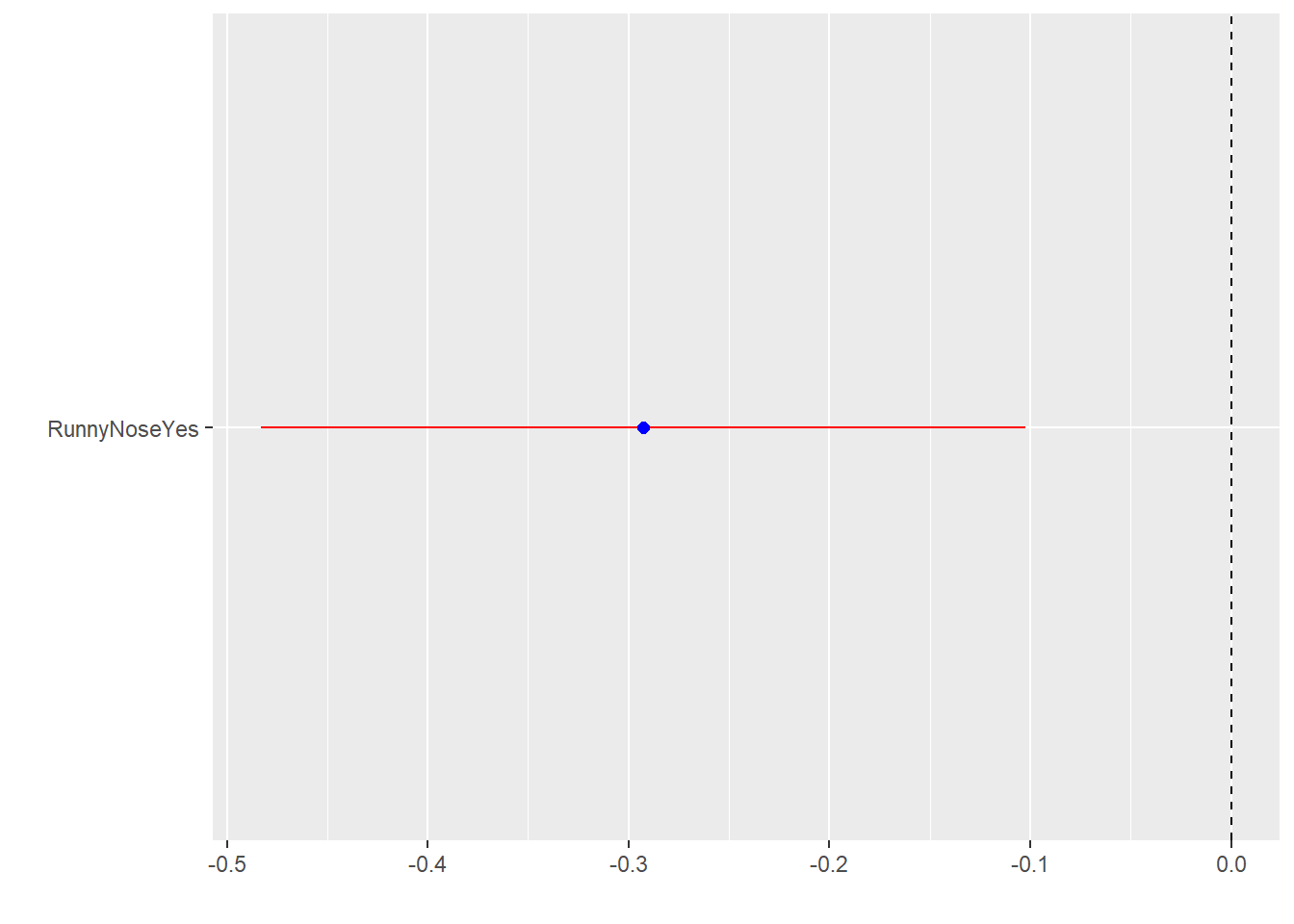
Model 1 Fitting a linear model. Body Temperature using only RunnyNose as predictor
<- %>% fit (BodyTemp ~ RunnyNose,data = Clean_df)
parsnip model object


Call:
stats::lm(formula = BodyTemp ~ RunnyNose, data = data)

Coefficients:
 (Intercept)  RunnyNoseYes
     99.1431       -0.2926
#Using the tidy function to get a better organized view of the result
# A tibble: 2 × 5
  term         estimate std.error statistic p.value
  <chr>           <dbl>     <dbl>     <dbl>   <dbl>
1 (Intercept)    99.1      0.0819   1210.   0
2 RunnyNoseYes   -0.293    0.0971     -3.01 0.00268
#we can also show the regression table results with dot and whisker plot
tidy (model1) %>% dwplot (dot_args = list (size= 2 ,color= "Blue" ),whisker_args = list (color= "Red" ),vline= geom_vline (xintercept = 0 ,color= "Black" ,linetype= 2 ))
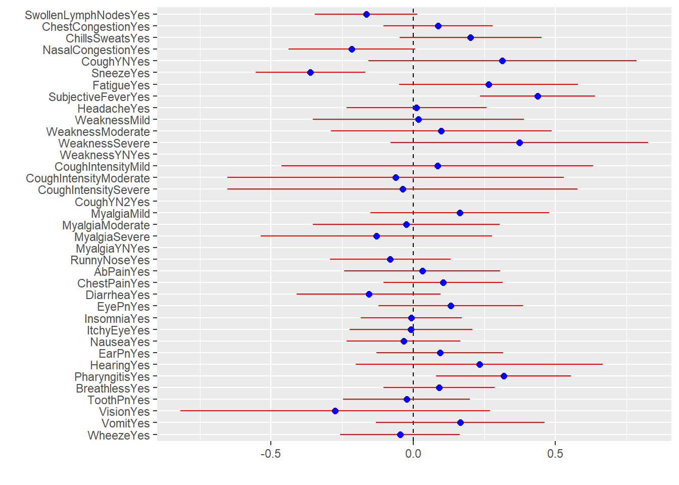
Model 2 Fitting Body Temperature using ALL predictors
<- %>% fit (BodyTemp ~ .,data= Clean_df)
parsnip model object


Call:
stats::lm(formula = BodyTemp ~ ., data = data)

Coefficients:
           (Intercept)    SwollenLymphNodesYes      ChestCongestionYes
             97.925243               -0.165302                0.087326
       ChillsSweatsYes      NasalCongestionYes              CoughYNYes
              0.201266               -0.215771                0.313893
             SneezeYes              FatigueYes      SubjectiveFeverYes
             -0.361924                0.264762                0.436837
           HeadacheYes            WeaknessMild        WeaknessModerate
              0.011453                0.018229                0.098944
        WeaknessSevere           WeaknessYNYes      CoughIntensityMild
              0.373435                      NA                0.084881
CoughIntensityModerate    CoughIntensitySevere             CoughYN2Yes
             -0.061384               -0.037272                      NA
           MyalgiaMild         MyalgiaModerate           MyalgiaSevere
              0.164242               -0.024064               -0.129263
          MyalgiaYNYes            RunnyNoseYes               AbPainYes
                    NA               -0.080485                0.031574
          ChestPainYes             DiarrheaYes                EyePnYes
              0.105071               -0.156806                0.131544
           InsomniaYes             ItchyEyeYes               NauseaYes
             -0.006824               -0.008016               -0.034066
              EarPnYes              HearingYes          PharyngitisYes
              0.093790                0.232203                0.317581
         BreathlessYes              ToothPnYes               VisionYes
              0.090526               -0.022876               -0.274625
              VomitYes               WheezeYes
              0.165272               -0.046665
# A tibble: 38 × 5
   term                 estimate std.error statistic   p.value
   <chr>                   <dbl>     <dbl>     <dbl>     <dbl>
 1 (Intercept)           97.9       0.304   322.     0
 2 SwollenLymphNodesYes  -0.165     0.0920   -1.80   0.0727
 3 ChestCongestionYes     0.0873    0.0975    0.895  0.371
 4 ChillsSweatsYes        0.201     0.127     1.58   0.114
 5 NasalCongestionYes    -0.216     0.114    -1.90   0.0584
 6 CoughYNYes             0.314     0.241     1.30   0.193
 7 SneezeYes             -0.362     0.0983   -3.68   0.000249
 8 FatigueYes             0.265     0.161     1.65   0.0996
 9 SubjectiveFeverYes     0.437     0.103     4.22   0.0000271
10 HeadacheYes            0.0115    0.125     0.0913 0.927
# … with 28 more rows
# ℹ Use `print(n = ...)` to see more rows
#We can also show the regression table results with dot and whisker plot
tidy (model2) %>% dwplot (dot_args = list (size= 2 ,color= "Blue" ),whisker_args = list (color= "Red" ),vline= geom_vline (xintercept = 0 ,color= "Black" ,linetype= 2 ))
#Compare model1 and model2, which model performs better?
compare_performance (model1,model2)
# Comparison of Model Performance Indices

Name   | Model |      AIC | AIC weights |      BIC | BIC weights |    R2 | R2 (adj.) |  RMSE | Sigma
----------------------------------------------------------------------------------------------------
model1 |   _lm | 2329.346 |    2.89e-06 | 2343.125 |        1.00 | 0.012 |     0.011 | 1.188 | 1.190
model2 |   _lm | 2303.840 |       1.000 | 2469.189 |    4.22e-28 | 0.129 |     0.086 | 1.116 | 1.144
Conclusion If looking at the R2 it looks like Model2 is a better fit than model1. However, if based on AIC, modle1 seems to be a better fit than model 2.
*Logistic Regression #Model 1 #Outcome=Nausea, Predictor=RunnyNose
<- logistic_reg ()%>% set_engine ("glm" )
<- glm_model %>% fit (Nausea ~ RunnyNose, data= Clean_df)
parsnip model object


Call:  stats::glm(formula = Nausea ~ RunnyNose, family = stats::binomial,
    data = data)

Coefficients:
 (Intercept)  RunnyNoseYes
    -0.65781       0.05018

Degrees of Freedom: 729 Total (i.e. Null);  728 Residual
Null Deviance:      944.7
Residual Deviance: 944.6    AIC: 948.6
#Get a better organized look of the result
# A tibble: 2 × 5
  term         estimate std.error statistic    p.value
  <chr>           <dbl>     <dbl>     <dbl>      <dbl>
1 (Intercept)   -0.658      0.145    -4.53  0.00000589
2 RunnyNoseYes   0.0502     0.172     0.292 0.770
<- glm_model %>% fit (Nausea ~ ., data= Clean_df)
parsnip model object


Call:  stats::glm(formula = Nausea ~ ., family = stats::binomial, data = data)

Coefficients:
           (Intercept)    SwollenLymphNodesYes      ChestCongestionYes
              0.222870               -0.251083                0.275554
       ChillsSweatsYes      NasalCongestionYes              CoughYNYes
              0.274097                0.425817               -0.140423
             SneezeYes              FatigueYes      SubjectiveFeverYes
              0.176724                0.229062                0.277741
           HeadacheYes            WeaknessMild        WeaknessModerate
              0.331259               -0.121606                0.310849
        WeaknessSevere           WeaknessYNYes      CoughIntensityMild
              0.823187                      NA               -0.220794
CoughIntensityModerate    CoughIntensitySevere             CoughYN2Yes
             -0.362678               -0.950544                      NA
           MyalgiaMild         MyalgiaModerate           MyalgiaSevere
             -0.004146                0.204743                0.120758
          MyalgiaYNYes            RunnyNoseYes               AbPainYes
                    NA                0.045324                0.939304
          ChestPainYes             DiarrheaYes                EyePnYes
              0.070777                1.063934               -0.341991
           InsomniaYes             ItchyEyeYes                EarPnYes
              0.084175               -0.063364               -0.181719
            HearingYes          PharyngitisYes           BreathlessYes
              0.323052                0.275364                0.526801
            ToothPnYes               VisionYes                VomitYes
              0.480649                0.125498                2.458466
             WheezeYes                BodyTemp
             -0.304435               -0.031246

Degrees of Freedom: 729 Total (i.e. Null);  695 Residual
Null Deviance:      944.7
Residual Deviance: 751.5    AIC: 821.5
#Get a better organized look of the result
# A tibble: 38 × 5
   term                 estimate std.error statistic p.value
   <chr>                   <dbl>     <dbl>     <dbl>   <dbl>
 1 (Intercept)             0.223     7.83     0.0285  0.977
 2 SwollenLymphNodesYes   -0.251     0.196   -1.28    0.200
 3 ChestCongestionYes      0.276     0.213    1.30    0.195
 4 ChillsSweatsYes         0.274     0.288    0.952   0.341
 5 NasalCongestionYes      0.426     0.255    1.67    0.0944
 6 CoughYNYes             -0.140     0.519   -0.271   0.787
 7 SneezeYes               0.177     0.210    0.840   0.401
 8 FatigueYes              0.229     0.372    0.616   0.538
 9 SubjectiveFeverYes      0.278     0.225    1.23    0.218
10 HeadacheYes             0.331     0.285    1.16    0.245
# … with 28 more rows
# ℹ Use `print(n = ...)` to see more rows
#Comparing the two logistic regression models for performance
compare_performance (glmmodel1,glmmodel2)
Warning in predict.lm(object, newdata, se.fit, scale = 1, type = if (type == :
prediction from a rank-deficient fit may be misleading

Warning in predict.lm(object, newdata, se.fit, scale = 1, type = if (type == :
prediction from a rank-deficient fit may be misleading

Warning in predict.lm(object, newdata, se.fit, scale = 1, type = if (type == :
prediction from a rank-deficient fit may be misleading
# Comparison of Model Performance Indices

Name      | Model |     AIC | AIC weights |     BIC | BIC weights | Tjur's R2 |  RMSE | Sigma | Log_loss | Score_log | Score_spherical |   PCP
----------------------------------------------------------------------------------------------------------------------------------------------
glmmodel1 |  _glm | 948.566 |    2.52e-28 | 957.752 |       1.000 | 1.169e-04 | 0.477 | 1.139 |    0.647 |  -107.871 |           0.012 | 0.545
glmmodel2 |  _glm | 821.471 |        1.00 | 982.227 |    4.84e-06 |     0.247 | 0.414 | 1.040 |    0.515 |      -Inf |           0.002 | 0.658
Logistic Regression Conclusion Based on model quality indicators such as AIC, model1 seems to be a better fit than model2