The below data was retrieved from the Global Adult Tobacco Survey website (Dataset for African Region, Botswana, Botswana - National ). The data was collected in 2017 in Botswana among adults 15 years and older. Both smokers and non smokers participated in the survey. a total of 4643 participated in this survey, a subset of 463 participants are used in this analysis. The below are unweighted calculations . The code book(BOT_GATS_207…) is located in the data_analysis_exercise folder.
Objective
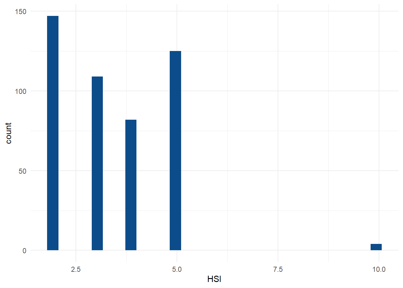
The objective of this analysis is to see if Gender predicts nicotine dependence. Only smokers were included in this analysis. Heavy Smoking Indeix(HSI) re:nicotine dependence was calculated as a score by adding B01+B07 variables.The scores were categorized as low addicition if score is between 0 and 2, and medium/high addiction score if between 3 and 6.
This uses MS Word as output format. See here for more information. You can switch to other formats, like html or pdf. See the Quarto documentation for other formats.
Data import and cleaning
Warning: package 'dplyr' was built under R version 4.2.2
Warning: package 'skimr' was built under R version 4.2.2
Warning: package 'memisc' was built under R version 4.2.2
Warning: package 'ggplot2' was built under R version 4.2.2
Warning: package 'labelled' was built under R version 4.2.2
#subsetting for variables of interest see bodebook. #A01 Gender, B01 smoking status, B04 age of smoking initiation, B07 smoking how soonafter awaking up, B06A number of cigarettes smoked
#checking my variables names of interest are selected and their strucutre
names(Bselect)
[1] "A01" "B01" "B04" "B07" "B06A"
str(Bselect)
tibble [4,643 × 5] (S3: tbl_df/tbl/data.frame)
 $ A01 : dbl+lbl [1:4643] 1, 1, 1, 1, 1, 1, 1, 1, 1, 1, 1, 1, 1, 1, 1, 1, 1, 1,...
   ..@ label      : chr "A01.  [RECORD GENDER FROM OBSERVATION.  ASK IF NECESSARY.]"
   ..@ format.spss: chr "F8.0"
   ..@ labels     : Named num [1:2] 1 2
   .. ..- attr(*, "names")= chr [1:2] "MALE" "FEMALE"
 $ B01 : dbl+lbl [1:4643] 3, 3, 3, 3, 3, 3, 3, 3, 3, 3, 3, 3, 3, 3, 3, 1, 2, 3,...
   ..@ label      : chr "B01.  Do you currently smoke tobacco on a daily basis, less than daily, or not at all?"
   ..@ format.spss: chr "F8.0"
   ..@ labels     : Named num [1:5] 1 2 3 7 9
   .. ..- attr(*, "names")= chr [1:5] "DAILY" "LESS THAN DAILY" "NOT AT ALL" "DON'T KNOW" ...
 $ B04 : num [1:4643] NA NA NA NA NA NA NA NA NA NA ...
  ..- attr(*, "label")= chr "B04.  How old were you when you first started smoking tobacco daily?  [IF DON'T KNOW OR REFUSED, ENTER 99]"
  ..- attr(*, "format.spss")= chr "F10.0"
 $ B07 : dbl+lbl [1:4643] NA, NA, NA, NA, NA, NA, NA, NA, NA, NA, NA, NA, NA, N...
   ..@ label      : chr "B07.  How soon after you wake up do you usually have your first smoke?  Would you say within 5 minutes, 6 to 30 minutes,"
   ..@ format.spss: chr "F8.0"
   ..@ labels     : Named num [1:5] 1 2 3 4 9
   .. ..- attr(*, "names")= chr [1:5] "WITHIN 5 MINUTES" "6 TO 30 MINUTES" "31 TO 60 MINUTES" "MORE THAN 60 MINUTES" ...
 $ B06A: num [1:4643] NA NA NA NA NA NA NA NA NA NA ...
  ..- attr(*, "label")= chr "B06A.  On average, how many of the following products do you currently smoke each day?  Also, let me know if you smoke t"
  ..- attr(*, "format.spss")= chr "F10.0"
#labeling my variable names
my_labels <-c(A01 ="Gender",B01 ="Do you currenlty smoke?",B04 ="How old were you when you frist started smoking?",B07 ="How soon do you smoke after you wake up",B06A="How many cigarattes do you smoke each day?")
print(my_labels)
                                               A01
                                          "Gender"
                                               B01
                         "Do you currenlty smoke?"
                                               B04
"How old were you when you frist started smoking?"
                                               B07
         "How soon do you smoke after you wake up"
                                              B06A
      "How many cigarattes do you smoke each day?"
#trying to set the variable name in the df but it didnt work
Found more than one class "haven_labelled" in cache; using the first, from namespace 'haven'
Also defined by 'memisc'
Found more than one class "haven_labelled" in cache; using the first, from namespace 'haven'
Also defined by 'memisc'
   Min. 1st Qu.  Median    Mean 3rd Qu.    Max.
  1.000   3.000   3.000   2.764   3.000   3.000
#creating a subset for smokers only based on B01 Do you currently smoke? only interested in responses 1,2 only (for daily and less than daily)
subset(Bselect, B01<=2)
# A tibble: 631 × 5
   A01       B01                   B04 B07                    B06A
   <dbl+lbl> <dbl+lbl>           <dbl> <dbl+lbl>             <dbl>
 1 1 [MALE]  1 [DAILY]              16  2 [6 TO 30 MINUTES]      5
 2 1 [MALE]  2 [LESS THAN DAILY]    NA NA                       NA
 3 1 [MALE]  1 [DAILY]              18  2 [6 TO 30 MINUTES]      5
 4 1 [MALE]  1 [DAILY]              14  2 [6 TO 30 MINUTES]      4
 5 1 [MALE]  1 [DAILY]              17  1 [WITHIN 5 MINUTES]     1
 6 1 [MALE]  2 [LESS THAN DAILY]    NA NA                       NA
 7 1 [MALE]  2 [LESS THAN DAILY]    NA NA                       NA
 8 1 [MALE]  2 [LESS THAN DAILY]    NA NA                       NA
 9 1 [MALE]  1 [DAILY]              19  2 [6 TO 30 MINUTES]     15
10 1 [MALE]  1 [DAILY]              20  3 [31 TO 60 MINUTES]     2
# … with 621 more rows
# ℹ Use `print(n = ...)` to see more rows
#saving the above as your dataset
Bselect2=subset(Bselect, B01<=2)
summary(Bselect2)
      A01             B01            B04             B07
 Min.   :1.000   Min.   :1.00   Min.   : 1.00   Min.   :1.000
 1st Qu.:1.000   1st Qu.:1.00   1st Qu.:17.50   1st Qu.:1.000
 Median :1.000   Median :1.00   Median :20.00   Median :2.000
 Mean   :1.165   Mean   :1.26   Mean   :28.83   Mean   :2.456
 3rd Qu.:1.000   3rd Qu.:2.00   3rd Qu.:25.50   3rd Qu.:4.000
 Max.   :2.000   Max.   :2.00   Max.   :99.00   Max.   :9.000
                                NA's   :164     NA's   :164
      B06A
 Min.   :  0.00
 1st Qu.:  1.00
 Median :  4.00
 Mean   : 27.85
 3rd Qu.:  6.00
 Max.   :999.00
 NA's   :164
#creting the HSI variable by adding B01 and B07,
Bselect2$HSI<-Bselect2$B01 + Bselect2$B07
#check if your variable has been calculated/ added
dim(Bselect2)
[1] 631 6
names(Bselect2)
[1] "A01" "B01" "B04" "B07" "B06A" "HSI"
str(Bselect2)
tibble [631 × 6] (S3: tbl_df/tbl/data.frame)
 $ A01 : dbl+lbl [1:631] 1, 1, 1, 1, 1, 1, 1, 1, 1, 1, 1, 1, 1, 1, 1, 1, 1, 1, ...
   ..@ label      : chr "Gender"
   ..@ format.spss: chr "F8.0"
   ..@ labels     : Named num [1:2] 1 2
   .. ..- attr(*, "names")= chr [1:2] "MALE" "FEMALE"
 $ B01 : dbl+lbl [1:631] 1, 2, 1, 1, 1, 2, 2, 2, 1, 1, 1, 1, 1, 1, 1, 1, 2, 1, ...
   ..@ label      : chr "Do you currenlty smoke?"
   ..@ format.spss: chr "F8.0"
   ..@ labels     : Named num [1:5] 1 2 3 7 9
   .. ..- attr(*, "names")= chr [1:5] "DAILY" "LESS THAN DAILY" "NOT AT ALL" "DON'T KNOW" ...
 $ B04 : num [1:631] 16 NA 18 14 17 NA NA NA 19 20 ...
  ..- attr(*, "label")= chr "How old were you when you frist started smoking?"
  ..- attr(*, "format.spss")= chr "F10.0"
 $ B07 : dbl+lbl [1:631]  2, NA,  2,  2,  1, NA, NA, NA,  2,  3,  1,  4,  4,  4...
   ..@ label      : chr "How soon do you smoke after you wake up"
   ..@ format.spss: chr "F8.0"
   ..@ labels     : Named num [1:5] 1 2 3 4 9
   .. ..- attr(*, "names")= chr [1:5] "WITHIN 5 MINUTES" "6 TO 30 MINUTES" "31 TO 60 MINUTES" "MORE THAN 60 MINUTES" ...
 $ B06A: num [1:631] 5 NA 5 4 1 NA NA NA 15 2 ...
  ..- attr(*, "label")= chr "How many cigarattes do you smoke each day?"
  ..- attr(*, "format.spss")= chr "F10.0"
 $ HSI : num [1:631] 3 NA 3 3 2 NA NA NA 3 4 ...
#check your new variable
Bselect2[1:500, ]
# A tibble: 500 × 6
   A01       B01                   B04 B07                    B06A   HSI
   <dbl+lbl> <dbl+lbl>           <dbl> <dbl+lbl>             <dbl> <dbl>
 1 1 [MALE]  1 [DAILY]              16  2 [6 TO 30 MINUTES]      5     3
 2 1 [MALE]  2 [LESS THAN DAILY]    NA NA                       NA    NA
 3 1 [MALE]  1 [DAILY]              18  2 [6 TO 30 MINUTES]      5     3
 4 1 [MALE]  1 [DAILY]              14  2 [6 TO 30 MINUTES]      4     3
 5 1 [MALE]  1 [DAILY]              17  1 [WITHIN 5 MINUTES]     1     2
 6 1 [MALE]  2 [LESS THAN DAILY]    NA NA                       NA    NA
 7 1 [MALE]  2 [LESS THAN DAILY]    NA NA                       NA    NA
 8 1 [MALE]  2 [LESS THAN DAILY]    NA NA                       NA    NA
 9 1 [MALE]  1 [DAILY]              19  2 [6 TO 30 MINUTES]     15     3
10 1 [MALE]  1 [DAILY]              20  3 [31 TO 60 MINUTES]     2     4
# … with 490 more rows
# ℹ Use `print(n = ...)` to see more rows
summary(Bselect2$HSI)
Min. 1st Qu. Median Mean 3rd Qu. Max. NA's
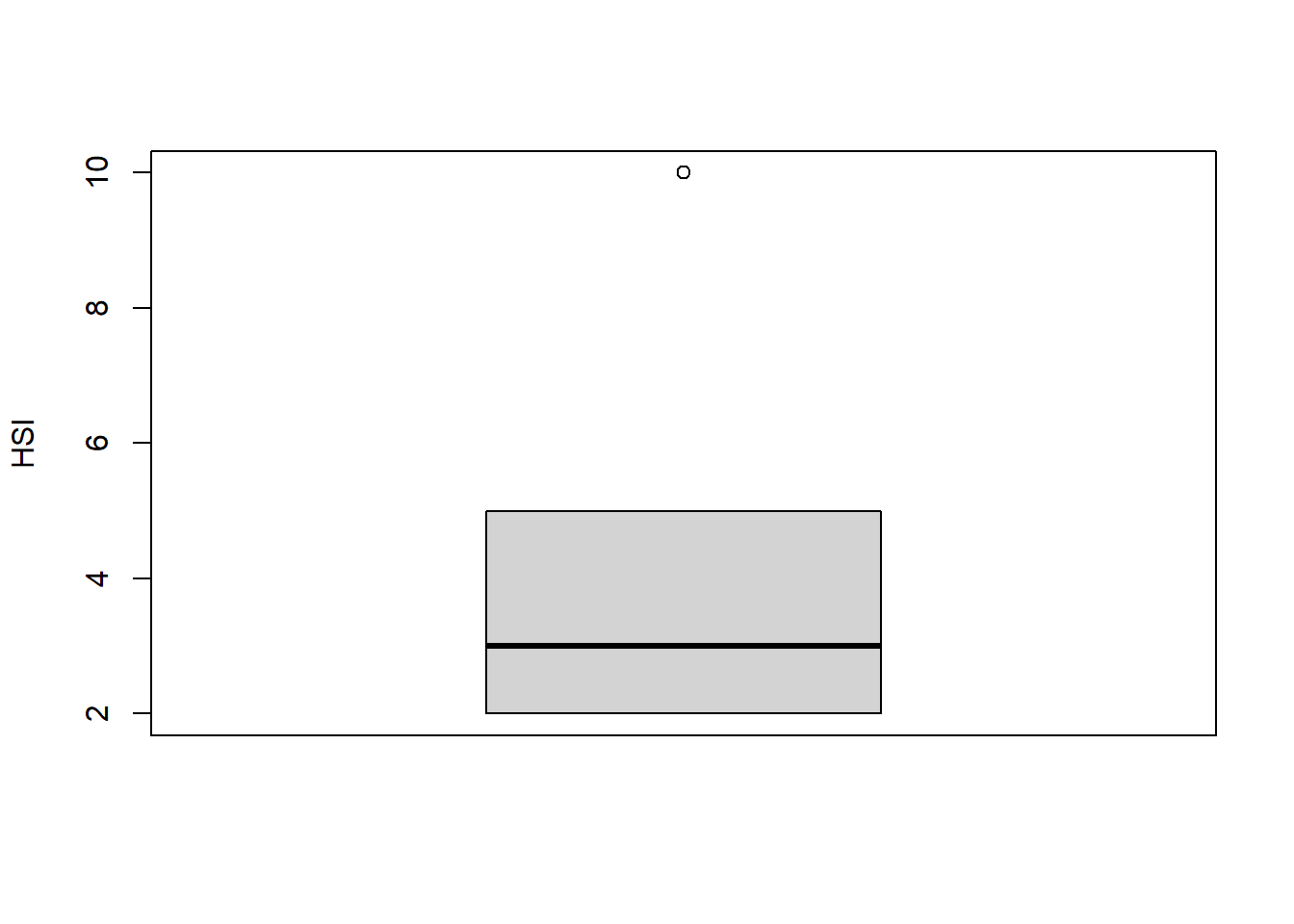
2.000 2.000 3.000 3.456 5.000 10.000 164
#remove missing by removig rows if HSI value is N/A
   Min. 1st Qu.  Median    Mean 3rd Qu.    Max.
  2.000   2.000   3.000   3.456   5.000  10.000
#NA is removed but there is an outlier as the max should only be 6, so removing the oulier. plotting a historgram and boxplot to see how many outliers there are
      A01              B01         B04             B07           B06A
 Min.   :0.0000   Min.   :1   Min.   : 1.00   Min.   :1.0   Min.   :  0.00
 1st Qu.:1.0000   1st Qu.:1   1st Qu.:17.00   1st Qu.:1.0   1st Qu.:  1.00
 Median :1.0000   Median :1   Median :20.00   Median :2.0   Median :  4.00
 Mean   :0.8467   Mean   :1   Mean   :28.56   Mean   :2.4   Mean   : 26.16
 3rd Qu.:1.0000   3rd Qu.:1   3rd Qu.:25.00   3rd Qu.:4.0   3rd Qu.:  6.00
 Max.   :1.0000   Max.   :1   Max.   :99.00   Max.   :4.0   Max.   :999.00
      HSI
 Min.   :0.0000
 1st Qu.:0.0000
 Median :1.0000
 Mean   :0.6825
 3rd Qu.:1.0000
 Max.   :1.0000
#save cleanted dataset as RDS
save(df_BSelect3,file="df_BSelect3.RDS")
To cite other work (important everywhere, but likely happens first in introduction), make sure your references are in the bibtex file specified in the YAML header above (here dataanalysis_template_references.bib) and have the right bibtex key. Then you can include like this:
Examples of reproducible research projects can for instance be found in [@mckay2020; @mckay2020a]
Methods
Describe your methods. That should describe the data, the cleaning processes, and the analysis approaches. You might want to provide a shorter description here and all the details in the supplement.
Data aquisition
As applicable, explain where and how you got the data. If you directly import the data from an online source, you can combine this section with the next.
Data import and cleaning
Write code that reads in the file and cleans it so it’s ready for analysis. Since this will be fairly long code for most datasets, it might be a good idea to have it in one or several R scripts. If that is the case, explain here briefly what kind of cleaning/processing you do, and provide more details and well documented code somewhere (e.g. as supplement in a paper). All materials, including files that contain code, should be commented well so everyone can follow along.
Statistical analysis
Explain anything related to your statistical analyses.
Results
Exploratory/Descriptive analysis
Use a combination of text/tables/figures to explore and describe your data. Show the most important descriptive results here. Additional ones should go in the supplement. Even more can be in the R and Quarto files that are part of your project.
Note the loading of the data providing a relative path using the ../../ notation. (Two dots means a folder up). You never want to specify an absolute path like C:\ahandel\myproject\results\ because if you share this with someone, it won’t work for them since they don’t have that path. You can also use the here R package to create paths. See examples of that below.
Basic statistical analysis
To get some further insight into your data, if reasonable you could compute simple statistics (e.g. simple models with 1 predictor) to look for associations between your outcome(s) and each individual predictor variable. Though note that unless you pre-specified the outcome and main exposure, any “p<0.05 means statistical significance” interpretation is not valid.
Full analysis
Use one or several suitable statistical/machine learning methods to analyze your data and to produce meaningful figures, tables, etc. This might again be code that is best placed in one or several separate R scripts that need to be well documented. You want the code to produce figures and data ready for display as tables, and save those. Then you load them here.
getwd()
Discussion
Summary and Interpretation
Summarize what you did, what you found and what it means.
Strengths and Limitations
Discuss what you perceive as strengths and limitations of your analysis.
Conclusions
What are the main take-home messages?
Include citations in your Rmd file using bibtex, the list of references will automatically be placed at the end
This paper [@leek2015] discusses types of analyses.
These papers [@mckay2020; @mckay2020a] are good examples of papers published using a fully reproducible setup similar to the one shown in this template.
Note that this cited reference will show up at the end of the document, the reference formatting is determined by the CSL file specified in the YAML header. Many more style files for almost any journal are available. You also specify the location of your bibtex reference file in the YAML. You can call your reference file anything you like, I just used the generic word references.bib but giving it a more descriptive name is probably better.