data_location <- here::here("fluanalysis","processed_data","Processed_data.Rds")

Processed_data <- readRDS(data_location)Model Evaluation
Load processed flu data file
#Install necessary packages
library(rsample) #for data splittingWarning: package 'rsample' was built under R version 4.2.2library(workflows) #for combining recipes and modelsWarning: package 'workflows' was built under R version 4.2.2library(tidymodels) # for the parsnip package, along with the rest of #tidy models Helper packagesWarning: package 'tidymodels' was built under R version 4.2.2── Attaching packages ────────────────────────────────────── tidymodels 1.0.0 ──✔ broom 1.0.1 ✔ purrr 0.3.4
✔ dials 1.1.0 ✔ recipes 1.0.5
✔ dplyr 1.1.0 ✔ tibble 3.1.8
✔ ggplot2 3.4.0 ✔ tidyr 1.2.0
✔ infer 1.0.4 ✔ tune 1.0.1
✔ modeldata 1.1.0 ✔ workflowsets 1.0.0
✔ parsnip 1.0.4 ✔ yardstick 1.1.0Warning: package 'dials' was built under R version 4.2.2Warning: package 'dplyr' was built under R version 4.2.2Warning: package 'ggplot2' was built under R version 4.2.2Warning: package 'infer' was built under R version 4.2.2Warning: package 'modeldata' was built under R version 4.2.2Warning: package 'parsnip' was built under R version 4.2.2Warning: package 'recipes' was built under R version 4.2.2Warning: package 'tune' was built under R version 4.2.2Warning: package 'workflowsets' was built under R version 4.2.2Warning: package 'yardstick' was built under R version 4.2.2── Conflicts ───────────────────────────────────────── tidymodels_conflicts() ──
✖ purrr::discard() masks scales::discard()
✖ dplyr::filter() masks stats::filter()
✖ dplyr::lag() masks stats::lag()
✖ recipes::step() masks stats::step()
• Learn how to get started at https://www.tidymodels.org/start/library(readr) # for importing data
Attaching package: 'readr'The following object is masked from 'package:yardstick':
specThe following object is masked from 'package:scales':
col_factorlibrary(broom.mixed) # for converting bayesian models to tidy tibblesWarning: package 'broom.mixed' was built under R version 4.2.2library(dotwhisker) # for visualizing regression resultsWarning: package 'dotwhisker' was built under R version 4.2.2library(dplyr)- #Split data into training dataset and test dataset
set.seed(222)
#select 3/4 of the data and save into training dataset
data_split <- initial_split(Processed_data, prop=3/4)
#now create the two data frames based on the above parameters
train_data <- training(data_split)
test_data <- testing(data_split)glimpse(Processed_data)Rows: 730
Columns: 32
$ SwollenLymphNodes <fct> Yes, Yes, Yes, Yes, Yes, No, No, No, Yes, No, Yes, Y…
$ ChestCongestion <fct> No, Yes, Yes, Yes, No, No, No, Yes, Yes, Yes, Yes, Y…
$ ChillsSweats <fct> No, No, Yes, Yes, Yes, Yes, Yes, Yes, Yes, No, Yes, …
$ NasalCongestion <fct> No, Yes, Yes, Yes, No, No, No, Yes, Yes, Yes, Yes, Y…
$ CoughYN <fct> Yes, Yes, No, Yes, No, Yes, Yes, Yes, Yes, Yes, No, …
$ Sneeze <fct> No, No, Yes, Yes, No, Yes, No, Yes, No, No, No, No, …
$ Fatigue <fct> Yes, Yes, Yes, Yes, Yes, Yes, Yes, Yes, Yes, Yes, Ye…
$ SubjectiveFever <fct> Yes, Yes, Yes, Yes, Yes, Yes, Yes, Yes, Yes, No, Yes…
$ Headache <fct> Yes, Yes, Yes, Yes, Yes, Yes, No, Yes, Yes, Yes, Yes…
$ Weakness <fct> Mild, Severe, Severe, Severe, Moderate, Moderate, Mi…
$ WeaknessYN <fct> Yes, Yes, Yes, Yes, Yes, Yes, Yes, Yes, Yes, Yes, Ye…
$ CoughIntensity <fct> Severe, Severe, Mild, Moderate, None, Moderate, Seve…
$ CoughYN2 <fct> Yes, Yes, Yes, Yes, No, Yes, Yes, Yes, Yes, Yes, Yes…
$ Myalgia <fct> Mild, Severe, Severe, Severe, Mild, Moderate, Mild, …
$ MyalgiaYN <fct> Yes, Yes, Yes, Yes, Yes, Yes, Yes, Yes, Yes, Yes, Ye…
$ RunnyNose <fct> No, No, Yes, Yes, No, No, Yes, Yes, Yes, Yes, No, No…
$ AbPain <fct> No, No, Yes, No, No, No, No, No, No, No, Yes, Yes, N…
$ ChestPain <fct> No, No, Yes, No, No, Yes, Yes, No, No, No, No, Yes, …
$ Diarrhea <fct> No, No, No, No, No, Yes, No, No, No, No, No, No, No,…
$ EyePn <fct> No, No, No, No, Yes, No, No, No, No, No, Yes, No, Ye…
$ Insomnia <fct> No, No, Yes, Yes, Yes, No, No, Yes, Yes, Yes, Yes, Y…
$ ItchyEye <fct> No, No, No, No, No, No, No, No, No, No, No, No, Yes,…
$ Nausea <fct> No, No, Yes, Yes, Yes, Yes, No, No, Yes, Yes, Yes, Y…
$ EarPn <fct> No, Yes, No, Yes, No, No, No, No, No, No, No, Yes, Y…
$ Hearing <fct> No, Yes, No, No, No, No, No, No, No, No, No, No, No,…
$ Pharyngitis <fct> Yes, Yes, Yes, Yes, Yes, Yes, Yes, No, No, No, Yes, …
$ Breathless <fct> No, No, Yes, No, No, Yes, No, No, No, Yes, No, Yes, …
$ ToothPn <fct> No, No, Yes, No, No, No, No, No, Yes, No, No, Yes, N…
$ Vision <fct> No, No, No, No, No, No, No, No, No, No, No, No, No, …
$ Vomit <fct> No, No, No, No, No, No, Yes, No, No, No, Yes, Yes, N…
$ Wheeze <fct> No, No, No, Yes, No, Yes, No, No, No, No, No, Yes, N…
$ BodyTemp <dbl> 98.3, 100.4, 100.8, 98.8, 100.5, 98.4, 102.5, 98.4, …Creating Model 1
Creating a recipe
flu_rec <-
  recipe(Nausea ~ ., data=train_data)
Creating a model
lr_mod<-
  logistic_reg()%>%
  set_engine("glm")
Combining the recipe and the model
flu_wflow <-
  workflow() %>%
  add_model(lr_mod)%>%
add_recipe(flu_rec)flu_wflow══ Workflow ════════════════════════════════════════════════════════════════════
Preprocessor: Recipe
Model: logistic_reg()
── Preprocessor ────────────────────────────────────────────────────────────────
0 Recipe Steps
── Model ───────────────────────────────────────────────────────────────────────
Logistic Regression Model Specification (classification)
Computational engine: glm flu_fit<-
flu_wflow %>%
fit(data=train_data)#to view your model details
flu_fit %>%
  extract_fit_parsnip() %>%
  tidy()
# A tibble: 38 × 5
term estimate std.error statistic p.value
<chr> <dbl> <dbl> <dbl> <dbl>
1 (Intercept) 1.63 9.40 0.173 0.862
2 SwollenLymphNodesYes -0.241 0.232 -1.04 0.298
3 ChestCongestionYes 0.219 0.257 0.853 0.394
4 ChillsSweatsYes 0.115 0.332 0.346 0.729
5 NasalCongestionYes 0.560 0.311 1.80 0.0713
6 CoughYNYes -0.705 0.611 -1.15 0.249
7 SneezeYes 0.117 0.248 0.473 0.636
8 FatigueYes 0.177 0.438 0.403 0.687
9 SubjectiveFeverYes 0.229 0.264 0.868 0.385
10 HeadacheYes 0.435 0.352 1.24 0.216
# … with 28 more rows
# ℹ Use `print(n = ...)` to see more rowsModel flu_fit evaluation
predict(flu_fit,test_data)Warning in predict.lm(object, newdata, se.fit, scale = 1, type = if (type == :
prediction from a rank-deficient fit may be misleading# A tibble: 183 × 1
.pred_class
<fct>
1 No
2 No
3 No
4 No
5 No
6 Yes
7 Yes
8 No
9 No
10 Yes
# … with 173 more rows
# ℹ Use `print(n = ...)` to see more rowsflu_aug <-
augment(flu_fit, test_data)Warning in predict.lm(object, newdata, se.fit, scale = 1, type = if (type == :
prediction from a rank-deficient fit may be misleading
Warning in predict.lm(object, newdata, se.fit, scale = 1, type = if (type == :
prediction from a rank-deficient fit may be misleadingflu_aug %>%
select (Nausea, RunnyNose,Fatigue,.pred_class,.pred_Yes)# A tibble: 183 × 5
Nausea RunnyNose Fatigue .pred_class .pred_Yes
<fct> <fct> <fct> <fct> <dbl>
1 No No Yes No 0.0377
2 Yes Yes Yes No 0.283
3 No Yes Yes No 0.320
4 Yes Yes Yes No 0.442
5 No No Yes No 0.170
6 Yes No Yes Yes 0.812
7 Yes Yes Yes Yes 0.746
8 No No Yes No 0.275
9 No No Yes No 0.280
10 Yes No Yes Yes 0.719
# … with 173 more rows
# ℹ Use `print(n = ...)` to see more rowsflu_aug %>%
roc_curve(truth=Nausea, .pred_No) %>%
autoplot()Warning: Returning more (or less) than 1 row per `summarise()` group was deprecated in
dplyr 1.1.0.
ℹ Please use `reframe()` instead.
ℹ When switching from `summarise()` to `reframe()`, remember that `reframe()`
always returns an ungrouped data frame and adjust accordingly.
ℹ The deprecated feature was likely used in the yardstick package.
Please report the issue at <https://github.com/tidymodels/yardstick/issues>.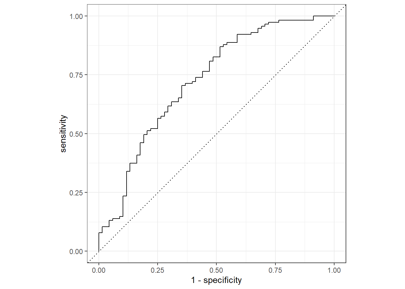
flu_aug %>%
  roc_auc(truth=Nausea, .pred_No)
# A tibble: 1 × 3
.metric .estimator .estimate
<chr> <chr> <dbl>
1 roc_auc binary 0.724Alternative Model
In this model we will fit only one predictor, our main predictor, the variable RunnyNose.
Creating a recipe
flu_recA <-
  recipe(Nausea ~ RunnyNose, data=train_data)
Creating a model
lr_mod<-
  logistic_reg()%>%
  set_engine("glm")
Combining the recipe and the model
flu_wflowA <-
  workflow() %>%
  add_model(lr_mod)%>%
add_recipe(flu_recA)flu_wflowA══ Workflow ════════════════════════════════════════════════════════════════════
Preprocessor: Recipe
Model: logistic_reg()
── Preprocessor ────────────────────────────────────────────────────────────────
0 Recipe Steps
── Model ───────────────────────────────────────────────────────────────────────
Logistic Regression Model Specification (classification)
Computational engine: glm flu_fitA<-
flu_wflowA %>%
fit(data=train_data)#to view your model details
flu_fitA %>%
  extract_fit_parsnip() %>%
  tidy()
# A tibble: 2 × 5
term estimate std.error statistic p.value
<chr> <dbl> <dbl> <dbl> <dbl>
1 (Intercept) -0.790 0.172 -4.59 0.00000447
2 RunnyNoseYes 0.188 0.202 0.930 0.352 Model flu_fit evaluation
predict(flu_fitA,test_data)# A tibble: 183 × 1
.pred_class
<fct>
1 No
2 No
3 No
4 No
5 No
6 No
7 No
8 No
9 No
10 No
# … with 173 more rows
# ℹ Use `print(n = ...)` to see more rowsflu_augA <-
augment(flu_fitA, test_data)flu_augA %>%
select (Nausea, RunnyNose,Fatigue,.pred_class,.pred_Yes)# A tibble: 183 × 5
Nausea RunnyNose Fatigue .pred_class .pred_Yes
<fct> <fct> <fct> <fct> <dbl>
1 No No Yes No 0.312
2 Yes Yes Yes No 0.354
3 No Yes Yes No 0.354
4 Yes Yes Yes No 0.354
5 No No Yes No 0.312
6 Yes No Yes No 0.312
7 Yes Yes Yes No 0.354
8 No No Yes No 0.312
9 No No Yes No 0.312
10 Yes No Yes No 0.312
# … with 173 more rows
# ℹ Use `print(n = ...)` to see more rowsflu_augA %>%
roc_curve(truth=Nausea, .pred_No) %>%
autoplot()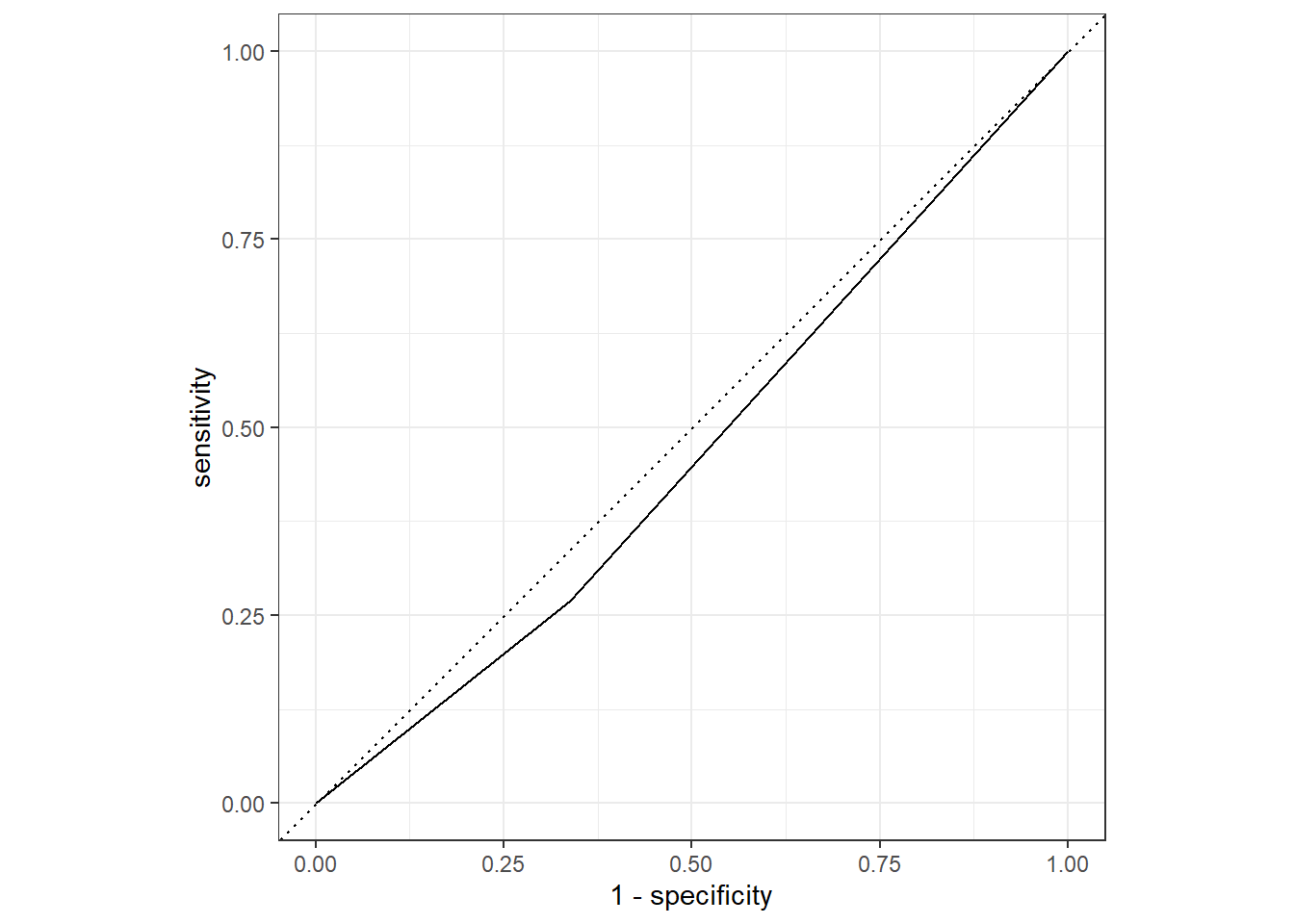
flu_augA %>%
  roc_auc(truth=Nausea, .pred_No)
# A tibble: 1 × 3
.metric .estimator .estimate
<chr> <chr> <dbl>
1 roc_auc binary 0.466Conclusion
From these model evaluation exercise, the first model where all predictors are used is a better fit. The roc_auc value is well over .5
The Alternative (Second model) where only RunnyNose variable is used as a predictor is NOT a good performing model. The roc_auc is under .5, and the graph seems like there is under fitting.
This section added by VIJAYPANTHAYI
I will be repeating the previous steps, however, instead fitting linear models to the continuous variable, body temperature. In order to do this. the metric needs to be changed to RMSE (root-mean-square-error).
#Create the training and test data sets from the original data set
set.seed(223)
data_split_linear <- initial_split(Processed_data,prop=3/4)
training_data_linear <- training(data_split_linear)
test_data_linear <- testing(data_split_linear)
Workflow Creation and Model Fitting
We will use tidymodels to generate our linear regression model. We will use recipe() and worklfow() to create the workflow.
# Initiate a new recipe
linear_recipe <- recipe(BodyTemp ~ ., data = training_data_linear)
# Create the linear regression model
linear <- linear_reg() %>%
             set_engine("lm")
# Create the workflow
flu_wflow_linear <-
      workflow() %>%
      add_model(linear) %>%
        add_recipe(linear_recipe)
flu_wflow_linear
══ Workflow ════════════════════════════════════════════════════════════════════
Preprocessor: Recipe
Model: linear_reg()
── Preprocessor ────────────────────────────────────────────────────────────────
0 Recipe Steps
── Model ───────────────────────────────────────────────────────────────────────
Linear Regression Model Specification (regression)
Computational engine: lm Model 2 Evaluation
Now that we have created the workflow, we can fit the model to the training and test data sets created previously.
training_fit_linear <- flu_wflow_linear %>%
                fit(data = training_data_linear)
test_fit_linear <- flu_wflow_linear %>%
                fit(data = test_data_linear)
The next step is to use the trained workflows, training_fit, to predict with unseen test data.
predict(training_fit_linear, test_data_linear)Warning in predict.lm(object = object$fit, newdata = new_data, type =
"response"): prediction from a rank-deficient fit may be misleading# A tibble: 183 × 1
.pred
<dbl>
1 99.4
2 98.8
3 99.8
4 98.8
5 98.4
6 99.9
7 99.2
8 98.9
9 99.1
10 99.4
# … with 173 more rows
# ℹ Use `print(n = ...)` to see more rowsWe now want to compare the estimates. To do this, we use augment().
training_aug_linear <- augment(training_fit_linear, training_data_linear)Warning in predict.lm(object = object$fit, newdata = new_data, type =
"response"): prediction from a rank-deficient fit may be misleadingtest_aug_linear <- augment(test_fit_linear, test_data_linear)Warning in predict.lm(object = object$fit, newdata = new_data, type =
"response"): prediction from a rank-deficient fit may be misleadingIf we want to assess how well the model makes predictions, we can use RMSE (root-mean-square-error) on the training_data and the test_data. RMSE is commonly used to evaluate the quality of predictions by measuring how far predictions fall from the measured true values. The lower the RMSE, the better the model.
training_aug_linear %>%
      rmse(BodyTemp, .pred)
# A tibble: 1 × 3
.metric .estimator .estimate
<chr> <chr> <dbl>
1 rmse standard 1.11Now, same for test_data.
test_aug_linear %>%
      rmse(BodyTemp, .pred)
# A tibble: 1 × 3
.metric .estimator .estimate
<chr> <chr> <dbl>
1 rmse standard 1.07The RMSE value for the training data set is 1.106 and the RMSE value for the test data set is 1.0666. This indicates that the model couldn’t find a solution or is not optimized very well for all predictors.
Alternative Model
Now, lets repeat these steps with only 1 predictor.
linear_recipe1 <- recipe(BodyTemp ~ RunnyNose, data = training_data_linear)

flu_wflow_linear1 <-
        workflow() %>%
        add_model(linear) %>%
        add_recipe(linear_recipe1)

training_fit_linear1 <- flu_wflow_linear1 %>%
        fit(data = training_data_linear)

test_fit_linear1 <- flu_wflow_linear1 %>%
        fit(data = test_data_linear)

training_aug_linear1 <- augment(training_fit_linear1, training_data_linear)
test_aug_linear1 <- augment(test_fit_linear1, test_data_linear)
Now, let’s find the RMSE for the training and test data sets.
training_aug_linear1 %>%
      rmse(BodyTemp, .pred)
# A tibble: 1 × 3
.metric .estimator .estimate
<chr> <chr> <dbl>
1 rmse standard 1.19Now, same for test_data.
test_aug_linear1 %>%
      rmse(BodyTemp, .pred)
# A tibble: 1 × 3
.metric .estimator .estimate
<chr> <chr> <dbl>
1 rmse standard 1.19The RMSE value for the training data set is 1.185 and the RMSE value for the test data set is 1.194. This still indicates that the model couldn’t find a solution or is not optimized very well for all predictors.
It appears that Model 1 predicts the categorical variable better than Model 2 predicts the continuous one.